[click anywhere
to close]
Background and Instructions
This tool computes cumulative CO
2 from excess CH
4 emissions, and vice versa. The idea is to illustrate that the famous ice core correlation of temperature and CO
2 can be reproduced solely by incremental CH
4 release at deglaciation. That is, the CO
2 curve is an effect of temperature change, not a cause. The source of this excess CH
4 is posited to be boreal/peat/tundra carbon buried by continuous snowfall at the onset of glaciation. This carbon is crushed, ground and anaerobically "fermented" by the increasing weight of ice, producing a methane-rich paste which is sequestered for thousands of years.
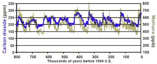
Correlation of methane and CO
2 emissions from the EPICA ice cores;
modified version of this
LBL original. Citation:
Schilt, A., et al. 2010. EPICA Dome C Ice Core 800KYr N2O Data. IGBP PAGES/World Data Center for Paleoclimatology Data Contribution Series # 2010-005. NOAA/NCDC Paleoclimatology Program, Boulder CO, USA. Accessed from the Carbon Dioxide Information Analysis Center, Oak Ridge National Laboratory, U.S. Department of Energy.
This model has these advantages. 1) The ice core data show a repetitive CO
2 cycle to only 280-300ppmv rather than a wider swing. The limit is reached because the system absorbs in proportion to the quantity present in the atmosphere and eventually a new, higher equilibrium is reached. The methane source is also more or less a fixed quantity, related to the carrying capacity of northern forests. 2) The phase relationship naturally appearing in ice cores, that of temperature change
preceding CO
2 change follows naturally from the fact that as glaciers melt back (due to
Milankovitch cycles) they expose and release the methane-saturated silt underneath. 3) As compared to the alternate hypothesis that warming causes release of CO
2 from the ocean, while true in part, this model has the advantage of producing a carbon isotope signature associated with land-plants, as has been found in ice cores.
The main tool computes absolute CO
2 levels from changing levels of methane, CH
4. Oxidation of methane produces CO
2 and water vapor. It assumes rates of CO
2 addition (CH
4 oxidation) and removal (weathering, ocean absorption, biomass accumulation) are directly proportional to their levels in the atmosphere. Similarly, it assumes the rates of stratospheric H
2O addition and removal are proportional to levels of CH
4 and H
2O, respectively.
The ODEs used are:

At the bottom of this tool is the "constants" section. The values should be self-explanatory by reference to the above equations.
CO2 absorption corresponds with
k1.
CH4 oxidation corresponds with
k2. Note that all CO
2 change is assumed to come from methane input - other sources and sinks are assumed in balance.
k2 also determines the rate of CH
4 depletion and stratospheric H
2O generation. This simple tool models
methane emissions as bimodal, thus there are two settings for
k3: "Normal" and "Elevated".
k4 is the rate of water vapor removal in the stratosphere.
Note: the tool originally modeled CH4 oxidation as primarily occurring in the stratosphere. However, neither where the oxidation occurs nor how fast the water vapor is removed changes the end result as the generated CO2 becomes well-mixed into the troposphere.
The simulation is assumed to start at the depths of a glacial cycle when a rise in insolation causes a glacial retreat. The retreat allows methane clathrates formed underneath the glacier to decompose, and the resulting meltwater runoff carries the methane from under the glacier to the surface. This runoff further facilitates the formation of boglands and other wetlands, which lead to a significant uptick in methane production, modeled here as a stepwise increase,
k3.
(Note: if the North American icesheets were 25 million km3 at their peak, the per annum meltwater flow could not have been less than 4X the current maximum flow of the Mississippi every year for 9000 yrs.) Oxidation of the methane produces CO
2 and H
2O vapor.
Note that the default rate of CO
2 removal, 0.00024/yr, corresponds to a half-life in the atmosphere of almost 3000 yrs, much longer than some current models predict for the present day. This does, however, correspond to the actual CO
2 levels as seen in ice core data which relax slowly. One possible explanation may be that the eruption of polar oceanic methane clathrates saturates the polar oceans with CO
2, altering the surface fugacity so that ocean absorption is much reduced.
H2O removal is determined by the rate of overturn of the stratosphere into the troposphere: 3-8 yrs, typically. The default value is a compromise to give observed levels of water in the stratosphere for "reasonable" values for other variables. Stratification is the ratio of stratospheric methane ppmv to that in the troposphere. It's tropospheric values that are captured in ice core data. However, the values used for CH
4 in the equations are total methane relative to the whole atmosphere, and have to be converted to and from sea-level (SL) values.
The second toolset, ΔCH
4 ↔ ΔCO
2 simply illustrates that an increase in CH4 emissions, from whatever source, can drive CO
2 from a glacial minimum of 180ppm to a interglacial maximum of 280ppm or more, if sustained for thousands of years. This is due to the relative longevity of CO
2 in the atmosphere. Note that this ultrasimplified tool unrealistically assumes infinite CO
2 longevity. The second half of this tool computes the inverse of the first calculation.
[click anywhere
to close]
Context
Milankovitch cycles may be the prime mover in deglaciation cycles, but positive feedbacks, in the form of
ice albedo and water vapor create
hysteresis in Earth's climate. That is, the world doesn't transition linearly from glacial to interglacial episodes, but flips between these states in a nonlinear and abrupt manner (much as thermostats are designed to do near their setpoints, to prevent the furnace from flickering on and off). This is why methane emissions are shown here as a step function, the simplest pedagogical model that captures the on-off (more-less) behavior of melt-driven emissions.
The most extreme examples of climate feedback have happened at least twice in Earth's history. At one extreme, the
"snowball Earth" hypothesis suggests that if glaciers advance far enough out of the polar regions, they will reflect so much sunlight that the Earth will continue to cool until nearly the entire planet is encapsulated in ice. It is believed that this happened at least once, prior to 650MyBP. At the other extreme, the
Paleocene-Eocene Thermal Maximum, or PETM occurred around 56MyBP, when the polar regions warmed dramatically and crocodiles could be found in southern Canada. In both cases positive feedbacks were certainly involved.
In addition to CO
2 and CH
4, another dramatic increase that occurred during the late 20th and early 21st centuries was in unfiltered coal particulates from China. During
La Niña conditions, the track of the polar jet stream runs up the western pacific and over Alaska, a track that runs coincidentally near to where the majority of seasonal polar ice cap melting has occurred, in the East Siberian, Chukchi and Beaufort seas. Fresh sea ice has a high albedo which can be dramatically reduced by windblown dust and soot, forming
"cryoconite", which concentrates in meltwater pools that absorb even more sunlight. China is replacing its coal power infrastructure with more modern plants, however, huge amounts of unfiltered residential cooking emissions will continue for decades to come.
Boreal Carbon
A key supposition in this argument is that there is enough carbon in boreal forests and soils to ultimately effect the carbon surge seen in ice core data. Here are some relevant statistics about the atmosphere. Its total mass is 5.15e18 kg. The constituents are typically given in molar "mixing ratios", including carbon dioxide, but for the purposes of this tool we need to convert those to mass units, ultimately gigatonnes, i.e., billions of metric tonnes.
| Component |
AMU |
Mixing ratio
(dry) |
Mass ratio
(wet) |
| N2 |
28 |
78.09% |
75.32% |
| O2 |
32 |
20.95% |
23.09% |
| Ar |
40 |
0.93% |
1.28% |
| H2O |
18 |
- |
0.25% |
| CO2 |
44 |
0.04% |
0.061% |
The total mass of CO
2 in the atmosphere is not 400 ppm of 5.15e18 kg, but 608 ppm by mass, or 3.13e15 kg = 3130 gigatonnes = 3130 Gt. When talking about soil carbon, the measurement is typically in Gt of just the carbon portion which is 12/44ths of 3130, or 854 Gt.
A typical change seen during deglaciation is from 180 to 280 ppmv, or 1/4 of the total amount of CO
2 currently in the atmosphere today, or around 213.5 Gt. So is there 213.5 Gt of carbon in the present-day forests of Alaska, Canada and Siberia? Short answer: yes.
The following chart is from the IPCC archives estimating carbon reserves and production in the various Earth biomes.
| Biome | Area
(109 ha) | | Global Carbon Stocks
(GtC) | Carbon density
(MgC/ha) | | | NPP
(GtC/yr) | |
|---|
| | WBGU | MRS | | WBGU | | MRS | IGBP | | | WBGU | MRS | IGBP | | Atjay | MRS | | |
| | | | | Plants | Soil | Total | Plants | Soil | Total | | Plants | Soil | Plants | Soil | |
| Tropical forests | 1.76 | 1.75 | | 212 | 216 | 428 | 340 | 213 | 553 | | 120 | 123 | 194 | 122 | | 13.7 | 21.9 | | |
| Temperate forests | 1.04 | 1.04 | | 59 | 100 | 159 | 139 | 153 | 292 | | 57 | 96 | 134 | 147 | | 6.5 | 8.1 | | |
| Boreal forests | 1.37 | 1.37 | | 88 | 471 | 559 | 57 | 338 | 395 | | 64 | 344 | 42 | 247 | | 3.2 | 2.6 | |
| Tropical savannas & grasslands | 2.25 | 2.76 | | 66 | 264 | 330 | 79 | 247 | 326 | | 29 | 117 | 29 | 90 | | 17.7 | 14.9 | | |
| Temperate grasslands & shrublands | 1.25 | 1.78 | | 9 | 295 | 304 | 23 | 176 | 199 | | 7 | 236 | 13 | 99 | | 5.3 | 7 | | |
| Deserts and semi-deserts | 4.55 | 2.77 | | 8 | 191 | 199 | 10 | 159 | 169 | | 2 | 42 | 4 | 57 | | 1.4 | 3.5 | | |
| Tundra | 0.95 | 0.56 | | 6 | 121 | 127 | 2 | 115 | 117 | | 6 | 127 | 4 | 206 | | 1 | 0.5 | | |
| Croplands | 1.6 | 1.35 | | 3 | 128 | 131 | 4 | 165 | 169 | | 2 | 80 | 3 | 122 | | 6.8 | 4.1 | | |
| Wetlands | 0.35 | - | | 15 | 225 | 240 | - | - | - | | 43 | 643 | - | - | | 4.3 | - | | |
|
| Total | 15.12 | 14.93 | | 466 | 2011 | 2477 | 654 | 1567 | 2221 | | | | | | | 59.9 | 62.6 | | |
Source: https://archive.ipcc.ch/ipccreports/tar/wg1/099.htm |
There are at two estimates each for the various parameters. Taking the lowest sum given for Boreal soil plus living plants yields 395 GtC - far in excess of the required 213.5 GtC, and this is
after the deglaciation when much of the accumulated
litterfall would have been converted to methane and released. Looking at it another way, and again taking the lowest value for
NPP or "Net Primary Production" gives 2.6 GtC
per year, or 44,200 GtC over a 17,000 interglacial. That number is too large for a number of reasons, for instance, because it neglects the ramp up and down in production as cold loosens and again tightens its grip, and because it neglects consumption by grazers. But cutting that number in half and half again still leaves >10,000 GtC with which to replenish the methane source. In fact, 10,000 GtC would be enough to supply
all methane produced at 0.4 GtCH4/yr ~ 0.3 GtC/yr for 17,000 years, or ~5100 GtC total.
What's unique about the Boreal biome is that, even though it has the second (or third) lowest productivity of all biomes, it covers a vast area that is kept in cold storage for much of the year. In fact, the whole of eastern Siberia is underlain by permafrost to this day, a lasting gift of the last glaciation. Material that falls to the ground here decomposes only slowly. Counterintuitively, once 2km of ice has built over a point, a geothermal flux of 80 mw/m
2 would require a surface temperature of -80C° to keep the base frozen. This only happens consistently in the highest, coldest parts or Antarctica, so in the boreal zone, the base of glaciers are unfrozen and able to support microbial life, even at the glacial maximum.
Another likely source of methane is the forests that grew in what are now temperate regions but during the depths of a glacial period would have a climate closer to that of Canada and Siberia. A portion of those forests would be drowned during deglaciation, with their decomposition contributing additional methane production.
Zoomed in: WAIS ice core data

Correlation of methane and CO
2 emissions from the WAIS ice cores;
Citations:
WAIS Temperature (lower-limit): Cuffey, K.M., G.D. Clow, E.J. Steig, C. Buizert, T.J. Fudge, M. Koutnik, E.D. Waddington,
R.B. Alley, and J.P. Severinghaus (2016). Deglacial temperature history of West Antarctica.
Proceedings of the National Academy of Sciences 113(50), 14249-14254.
doi: 10.1073/pnas.1609132113
CO2:
Marcott, S. et al. 2014. Centennial-scale changes in the global carbon cycle during the last deglaciation., Nature. 514. 616-619. https://doi.org/10.1038/nature13799
CH4:
Rachael H. Rhodes, Edward J. Brook, John C. H. Chiang, Thomas Blunier, Olivia J. Maselli, Joseph R. McConnell, Daniele Romanini, Jeffrey P. Severinghaus (2015-05-29)
Enhanced tropical methane production in response to iceberg discharge in the North Atlantic.
Science and
C. Buizert et al., The WAIS Divide deep ice core WD2014 chronology - Part 1: Methane synchronization (68-31 ka BP) and the gas age-ice age difference. Clim Past. 11, 153-173 (2015).
The problem with the far-inland ice cores of EPICA/Dome C and Vostok (etc) is that they receive very little snowfall. Though the resulting cores go back a long ways, the individual annual layers are too thin for fine-grained analysis. Although the Greenland ice cores received much more snowfall, they have more contaminants and are considered relatively "noisy".
For these reasons, ice cores from a region with higher annual snow fall, in the West Antarctic Ice Sheet (WAIS), were obtained and they resolve several outstanding questions.
First off, it's clear from the chart at left (above), that CO
2 is a consequence of deglaciation, not a driver. Although the trend lines are hand-drawn it's clear that temperature heads north as early as 22000 yBP (where "present" is defined as 1950). The plots for CO
2 and CH
4 are plotted versus
gas age, which delays them by ~200 yrs, but were they moved 200 yrs to the left it would not change this result.
Second, although this tool was developed with reference to the inland cores, the ratio between CO
2 and CH
4 holds, at least until the
Bølling-Allerød warm period, shown in pink, and the following
Younger Dryas cold relapse, shown in pale blue. On the plus side, the Bølling-Allerød warm period shows a huge burst of methane production, as would be expected if the collapse of northern ice sheets unleashed buried methane clathrates. On the downside, if you read this literally, methane looks to be an "
anti-greenhouse gas", which is a non-physical result, and it does not have the predicted effect on CO
2. Temperatures trend downwards until the Younger Dryas, despite CO
2 remaining constant and CH
4 at twice it's minimum level.
Although WAY outside the scope of this simple tool, the presumption is that this behavior is consistent with what ultimately
caused the Younger Dryas, namely that fresh meltwater from collapsing glacial dams, shutdown the
Gulf stream, cooling Europe to the point where snow would persist and positive albedo feedback would make it colder still, until all of the glacial meltwater was either exhausted or refrozen, at which point the Gulf stream rebooted. Consequently, the Northern Hemisphere exited the Younger Dryas with a vengeance and brought us into the warm Holocene present.
Glacial Cycles: Methane Oxidation copyright (C) Neon Media, LLC.
All rights reserved. This software is licensed, not sold.
THIS SOFTWARE IS PROVIDED BY THE COPYRIGHT HOLDERS AND CONTRIBUTORS "AS IS"
AND ANY EXPRESS OR IMPLIED WARRANTIES, INCLUDING, BUT NOT LIMITED TO, THE
IMPLIED WARRANTIES OF MERCHANTABILITY AND FITNESS FOR A PARTICULAR PURPOSE ARE
DISCLAIMED. IN NO EVENT SHALL NEON MEDIA, LLC, ITS PARTNERS, EMPLOYEES, OR ASSIGNS BE LIABLE FOR ANY DIRECT,
INDIRECT, INCIDENTAL, SPECIAL, EXEMPLARY, OR CONSEQUENTIAL DAMAGES (INCLUDING,
BUT NOT LIMITED TO, PROCUREMENT OF SUBSTITUTE GOODS OR SERVICES; LOSS OF USE,
DATA, OR PROFITS; OR BUSINESS INTERRUPTION) HOWEVER CAUSED AND ON ANY THEORY
OF LIABILITY, WHETHER IN CONTRACT, STRICT LIABILITY, OR TORT (INCLUDING
NEGLIGENCE OR OTHERWISE) ARISING IN ANY WAY OUT OF THE USE OF THIS SOFTWARE,
EVEN IF ADVISED OF THE POSSIBILITY OF SUCH DAMAGE.
Portions (D3.js and D3-format.js) copyright (C) 2010-2016, Michael Bostock.
All rights reserved.
Redistribution and use (of D3.js and D3-format.js) in source and binary forms, with or without
modification, are permitted provided that the following conditions are met:
* Redistributions of source code must retain the above copyright notice, this
list of conditions and the following disclaimer.
* Redistributions in binary form must reproduce the above copyright notice,
this list of conditions and the following disclaimer in the documentation
and/or other materials provided with the distribution.
* The name Michael Bostock may not be used to endorse or promote products
derived from this software without specific prior written permission.
THIS SOFTWARE IS PROVIDED BY THE COPYRIGHT HOLDERS AND CONTRIBUTORS "AS IS"
AND ANY EXPRESS OR IMPLIED WARRANTIES, INCLUDING, BUT NOT LIMITED TO, THE
IMPLIED WARRANTIES OF MERCHANTABILITY AND FITNESS FOR A PARTICULAR PURPOSE ARE
DISCLAIMED. IN NO EVENT SHALL MICHAEL BOSTOCK BE LIABLE FOR ANY DIRECT,
INDIRECT, INCIDENTAL, SPECIAL, EXEMPLARY, OR CONSEQUENTIAL DAMAGES (INCLUDING,
BUT NOT LIMITED TO, PROCUREMENT OF SUBSTITUTE GOODS OR SERVICES; LOSS OF USE,
DATA, OR PROFITS; OR BUSINESS INTERRUPTION) HOWEVER CAUSED AND ON ANY THEORY
OF LIABILITY, WHETHER IN CONTRACT, STRICT LIABILITY, OR TORT (INCLUDING
NEGLIGENCE OR OTHERWISE) ARISING IN ANY WAY OUT OF THE USE OF THIS SOFTWARE,
EVEN IF ADVISED OF THE POSSIBILITY OF SUCH DAMAGE.


